
Introduction
Today, we're rolling out the first part of a multi-part educational series on sampling, oversampling, and aliasing. When it's all out there, we'll be sharing the whole thing as a PDF for handy reading, along with a couple surprises... Let's get started with part 1!
Aliasing distortion, an unpleasant artifact of sampling audio, and oversampling, a process that increases the sample rate of audio, are very popular topics in forums, product marketing, and video tutorials. It’s no surprise! Here are three important reasons:
- Aliasing distortion is a fundamental challenge with digital audio. It sounds bad.
- Oversampling can reduce aliasing until it’s beneath the hearing threshold.
- Because oversampling is described with one number (2, 4, 8, etc.), it seems easy to understand and is easy to drop into marketing literature.
As it turns out, not all oversampling is the same. You don’t always need it, and developers face several trade-offs when implementing it. This series aims to help you understand aliasing distortion, how oversampling addresses it, and when to use oversampling.
Understanding Sampling
When I say sampling I mean that we have a continuous signal (physical reality) and we want to represent it using a finite amount of data, so we sample discrete (countable, individual) points along that signal, evenly spaced in time. Here’s a simplified description of how sound travels from the environment into your computer:
- The air carries continuous sound waves to the microphone.
- The air pushes the microphone diaphragm around, making it vibrate.
- The diaphragm moves a magnet, creating a modulating electric current.
- The current goes through an XLR cable into your audio interface, and is amplified by the microphone preamp.
- The preamp passes audio to the analog-to-digital converter (ADC), which grabs discrete values from the electric current at even intervals (the sample rate).*
- The sample values are passed from your interface to your computer, which saves them as an AIFF or WAV.
* This used to be a bit more straightforward, but over the years ADC and DAC converters use a more complicated process known as Delta-Sigma modulation to do this work. Detailing that is beyond the scope of this series for now.
The opposite happens on the way back. The discrete samples are fed back through a digital-to-analog converter (DAC), which reconstructs a continuous electric current from the samples and sends that to your speakers, which convert the current to a magnetic force to move the speaker cones. Voila: sound!
There are two degrees of precision we care about for each sample:
- Sample rate describes how many discrete samples the ADC takes of the continuous signal per second.
- Bit depth describes how precisely samples measure the strength of the signal.
In this series, we’re discussing the effects of samples over time, rather than the accuracy of each sample, so we’re going to talk about the sample rate.
How sampling causes aliasing
To recap: the sample rate determines how many discrete samples the ADC takes per second from a continuous signal. The main tradeoff when selecting a sample rate is:
- Lower rates use fewer samples and are easier to process and store.
- Higher rates use more samples and resources, but can represent higher frequencies in the signal.
The highest frequency that can be represented by any sample rate is called the Nyquist frequency (we’ll use Nyquist, for short). Lucky for us, the math to find Nyquist is easy: it’s 1/2 the sample rate! For 44,100 samples per second (44.1 kHz/CD quality), the highest frequency we can represent is about 22 kHz. Engineers picked this rate in the 1970’s because its Nyquist frequency is slightly higher than the highest frequency humans are known to hear. So how does any of this relate to aliasing?
Imagine we’re taking a video of somebody dribbling a basketball twice per second (2 Hz). If we’re filming at 12 frames per second (12 Hz), we could see the dribbles easily, twice per second:
0           1           2           3      Seconds
`````````````````````````````````````
-     -     -     -     -     -     -
 -   - -   - -   - -   - -   - -   -
  - -   - -   - -   - -   - -   - -
   -     -     -     -     -     -
`````````````````````````````````````
      1     2     3     4     5     6      Dribbles (2 Hz)
Even if the player started dribbling at 6hz, we could record the pattern accurately:
0           1           2           3      Seconds
`````````````````````````````````````
- - - - - - - - - - - - - - - - - - -


 - - - - - - - - - - - - - - - - - -
`````````````````````````````````````
  1 2 3 4 5 6...                           Dribbles (6 Hz)
We have a problem: as soon as the player dribbles any faster than 6 Hz, our second sample will happen after the ball has bounced and is headed back up. And the third might be after it went back up and is on the way down:
0                                          Seconds
`````````````````````````````````````
-    -      -
  --   -  -
 -  -   --
      -    -
`````````````````````````````````````
  1 2  3 4…                                Dribbles (>6 Hz)
Sampling does not record the direction of the ball, only its position in the air. So, we don’t know how to reconstruct the movement of the ball: at sample 2, is the ball still going down towards the ground, or is it bouncing up? Even worse, if the player dribbles at exactly the same speed as the sample rate, the ball doesn’t appear to move at all:
0           1           2           3      Seconds
`````````````````````````````````````
-------------------------------------


`````````````````````````````````````
 123456789…                                Dribbles (12 Hz)
It’s very similar to watching a wheel that spins faster and faster. Your brain can’t process it fast enough, so you start to see it slow down, stop, and eventually spin backwards… that’s aliasing happening directly in your brain!
Just like the wheel goes backwards, audio aliasing results in frequencies that have “bounced off” or “folded back over” the Nyquist frequency during sampling. Frequencies in the continuous signal immediately above Nyquist cause aliasing distortion in the sampled signal that is too high a frequency to hear. As the frequencies in the continuous signal get higher and higher, they eventually fold back into the audible range as inharmonic, metallic ringing in the sampled signal. That’s the sound of aliasing!
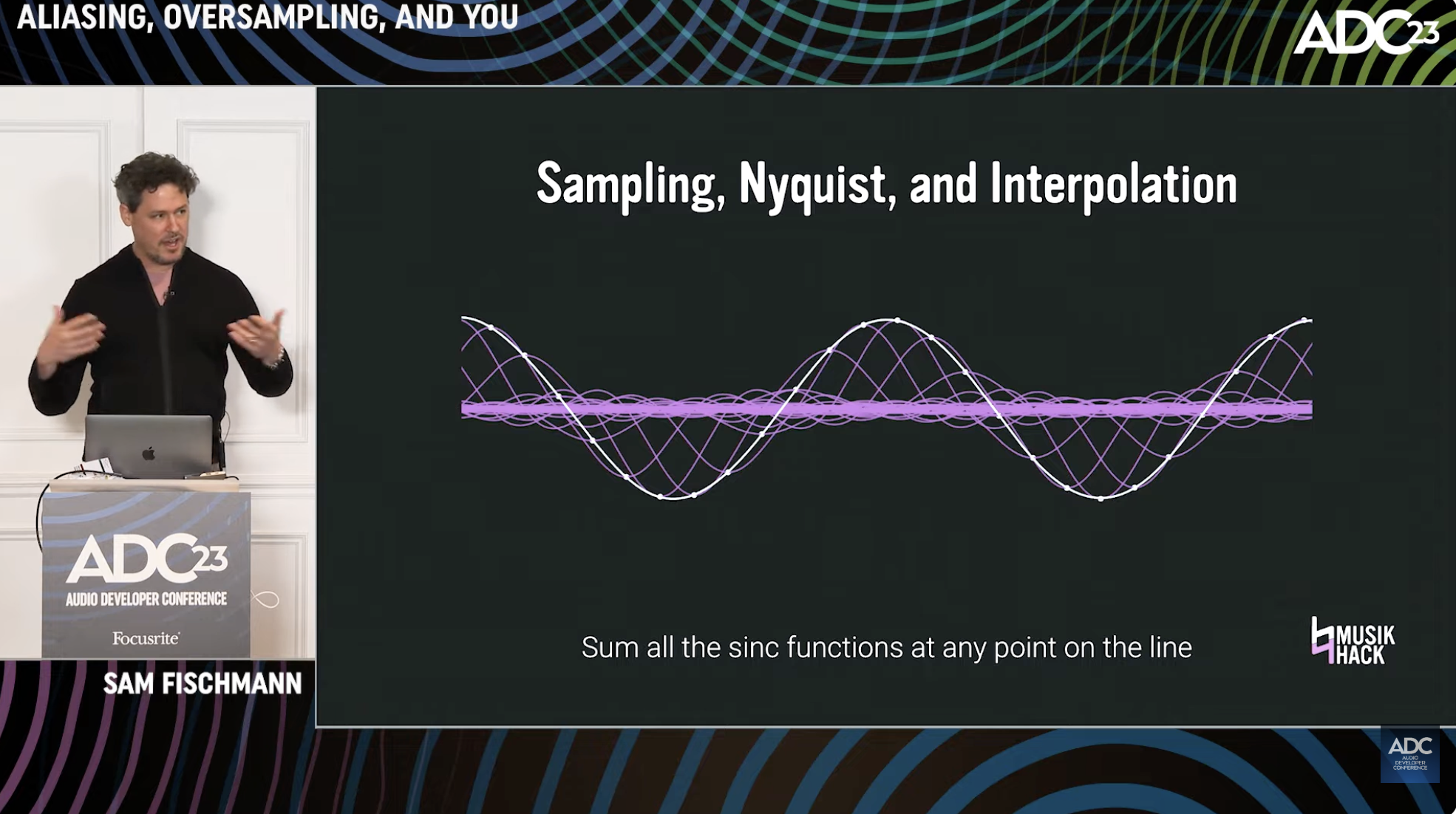
In audio, we rarely have a simple signal like we did in our ball example. We have very complex waveforms! There’s some brilliant math called Fourier’s theory, which shows us that we can think of any complex, periodic signal as a sum of many component sine waves, each with different frequencies, volumes, and phases. Depending on the literature and process being described, these components might be called:
- bands (we’ll use this term in a minute, take note)
- bins
- harmonics
- overtones
- timbre (when describing the sound of all components at once)
While the math of Fourier’s theory is beyond the scope of this series, it’s important to know that thinking about signals as sums of sine waves is very helpful. When a complex signal is sampled, the components below Nyquist frequency of the sampling rate are preserved, but those higher than Nyquist alias back towards zero.
Hope you've come away from this with some more understanding of what aliasing is and how it causes problems! Next week, we'll be back with part 2: the role of filters in sampling!